The innovative Early Warning System

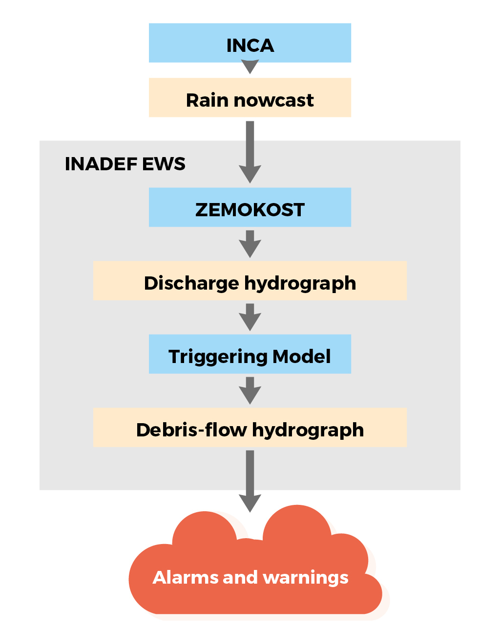
1. Runoff volume contributing to debris flow

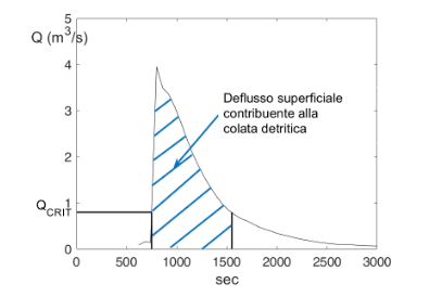
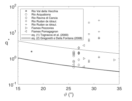
The runoff contributing volume to debris flow is that corresponding to the part of runoff hydrograph exceeding the critical discharge for the debris-flow generation (figure 1). Such a concept was initially introduced by Bennet et al. (2014), and later resumed by Gregoretti et al. (2016b). The critical discharge is the liquid discharge able to entrain the large quantity of sediments needed for the formation of a solid-liquid current (figure 2) and was firstly estimated by Tognacca et al. (2000) through an empirical relationship based on laboratory-flume experiments of debris-flow generation:

q_CRIT =4d_M^1.5 tanϑ^-1.17                      (1)

where q_CRIT is the unit width critical discharge, d_M the mean diameter of sediments and ϑ the bed slope angle. Gregoretti and Dalla Fontana (2008) proposed an analogous relationship based on laboratory flume experiments of the inception of high rate entrainment of sediments into water flow:

q_CRIT= 0.78 d_M^1.5 tanϑ^-1.27                     (2)

Equation (1) corresponds to a debris flow to be generated in a short distance, while equation (2) concerns the limit for the high rate sediment entrainment to have the generation of a debris flow. For these reasons, equation (1) provides values of q_CRIT about four times larger than equation (2). Moreover, Gregoretti and Dalla Fontana (2008) compared the estimates of the critical discharge provided by equation (2) with the simulated values of runoff peak discharge of about 30 debris-flow events occurred on the Dolomites in the period 1993-2006. Figure 3 shows that equation (2) in its dimensionless form, represents an inferior limit for the simulated peak discharge of all the events. Recently, Pastorello et al. (2020) proposed a relationship analogous to those of Tognacca et al. (2000) and Gregoretti and Dalla Fontana (2008) for the critical discharge corresponding to the occurrence of high magnitude debris flows.

The peak value of the solid-liquid discharge is computed according to the relationship provided by Takahashi (1978, 2007) and updated by Lanzoni et al. (2017) on a base of systematic series of debris flows generated in a laboratory flume:

 Q_P=0.75c*/(c*- c_F ) Q_PL   (3)

where Q_P is the peak solid-liquid discharge, c* is the dry bed sediment concentration, c_F is the sediment concentration at the front of the debris flow and Q_PL is the peak runoff discharge. This relationship is based on the mass conservation equation and assuming the maximum value allowed for c_F = 0.9 c* (Takahashi, 2007) the peak solid liquid discharge can grow up to 7.5 times of the peak runoff discharge. Field data shows that this amplification factor could be underestimated (Kean et al., 2016). In literature there are some relationships for the estimating c_F (Gregoretti and Degetto, 2012). Here that of Takahashi (1978) updated by Lanzoni et al. (2017) is shown:

c_F=tanϑ/((ρ_S/ρ-1)(tanϕ_qs-tanϑ))                                                                     (4)

where ϕ_qs is the quasi-static friction angle (ratio between shear and normal stresses in the region just over the static bed).

The solid-liquid volume,V_SL, is computed combining the runoff volume contributing to debris flow, VL (blue dashed area in figure 1), with or the sediment volume V_SED or the mean sediment concentration c. The sediment volume can be saturated and in this case:

V_SL = V_L+ V_SED = V_L + V_S/c*                         (5)

otherwise:

V_SL = V_L + (1 – c*)SV_S/c*                                 (6)

where V_S is the solid volume and S the saturation degree of the entrained sediments. Equations (5) and (6) can be written using the mean sediment concentration c (V_S/V_SL). Substituting V_S with c V_SL equations (5) and (6) becomes:

V_SL = V_L /(1 – c/c*)                                          (7)

V_SL = V_L /(1 – (1-S)c -cS/c*)                            (8)

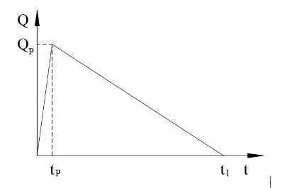
Known Q_P and V_SL the solid-liquid hydrograph is determined because its duration is fixed: tI = 2 V_SL/Q_P (figure 4).

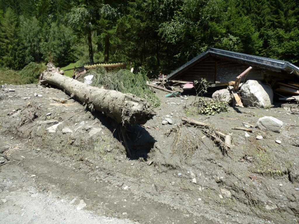
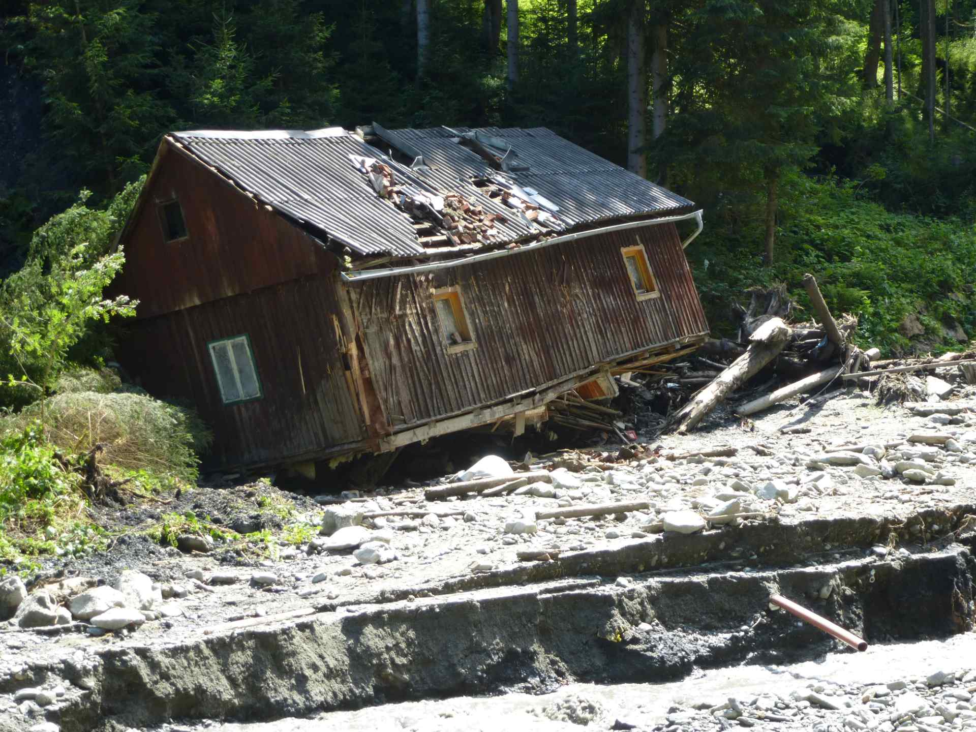
The value of Q_P is determined after the computation of Q_PL and c_F, known the characteristics of sediments (c*, ϕ_qs) and morphology (ϑ) in the initiation area. The value of V_SL is estimated also by V_S or c. These last values depend on the entrainment rate that increases with the peak runoff hydrograph and slope (Lanzoni et al. 2017) and on the length of the reach between the formation of the front and the reference location where the solid-liquid hydrograph should be estimated. In the case of Rovina di Cancia, the values of V_SED and c can be estimated using data of previously occurred debris flows (simulated runoff hydrographs and sediment volume entrained and deposited during  debris-flow routing). The analysis of data of the entrained volume of sediments on the reach between the altitude of 1666 m a.s.l. and the flat area at altitude of 1344 m a.s.l. (see the description of the site of Cancia) and the estimates of the runoff volume contributing to debris flow for the debris flows occurred on 18 July 2009, 23 July 2015, 4 August 2015, 1 July 2020 and 29 August 2020, provides an average value of c = 0.5 (0.38 < c < 0.56) after assuming S = 1 and c* = 0.62 (Gregoretti et al., 2019). This value is that to be used for the estimate of the sediments volume transported by the debris flow upstream the flat depositional area. The data of all the sediments volumes transported by the debris flows occurred on 1994-2020 show that it is 10000 m3 the value of the sediments volume retained by the flat deposition area and by the upstream reach.